github PyPI version license Documentation Status

Welcome to qnm¶

Python implementation of Cook-Zalutskiy spectral approach to computing Kerr quasinormal frequencies (QNMs).

With this python package, you can compute the QNMs labeled by different (s,l,m,n), at a desired dimensionless spin parameter 0≤a<1. The angular sector is treated as a spectral decomposition of spin-weighted spheroidal harmonics into spin-weighted spherical harmonics. Therefore the spherical-spheroidal decomposition coefficients come for free when solving for ω and A.

We have precomputed a large number of low-lying modes (s=-2 and s=-1, all l<8, all n<7). These can be automatically installed with a single function call, and interpolated for good initial guesses for root-finding at some value of a.

Installation¶

PyPI¶

qnm is available through PyPI:

pip install qnm

From source¶

git clone https://github.com/duetosymmetry/qnm.git
cd qnm
python setup.py install

If you do not have root permissions, replace the last step with python setup.py install --user

Dependencies¶

All of these can be installed through pip or conda.

numpy
scipy
numba
tqdm (just for qnm.download_data() progress)

Documentation¶

Automatically-generated API documentation is available on Read the Docs: qnm.

Usage¶

The highest-level interface is via qnm.cached.KerrSeqCache, which loads cached spin sequences from disk. A spin sequence is just a mode labeled by (s,l,m,n), with the spin a ranging from a=0 to some maximum, e.g. 0.9995. A large number of low-lying spin sequences have been precomputed and are available online. The first time you use the package, download the precomputed sequences:

import qnm

qnm.download_data() # Only need to do this once
# Trying to fetch https://duetosymmetry.com/files/qnm/data.tar.bz2
# Trying to decompress file /<something>/qnm/data.tar.bz2
# Data directory /<something>/qnm/data contains 860 pickle files

Then, use qnm.cached.KerrSeqCache to load a qnm.spinsequence.KerrSpinSeq of interest. If the mode is not available, it will try to compute it (see detailed documentation for how to control that calculation).

ksc = qnm.cached.KerrSeqCache(init_schw=True) # Only need init_schw once
mode_seq = ksc(s=-2,l=2,m=2,n=0)
omega, A, C = mode_seq(a=0.68)
print(omega)
# (0.5239751042900845-0.08151262363119974j)

Calling a spin sequence with mode_seq(a) will return the complex quasinormal mode frequency omega, the complex angular separation constant A, and a vector C of coefficients for decomposing the associated spin-weighted spheroidal harmonics as a sum of spin-weighted spherical harmonics.

Visual inspections of modes are very useful to check if the solver is behaving well. This is easily accomplished with matplotlib. Here are some simple examples:

import numpy as np
import matplotlib as mpl
import matplotlib.pyplot as plt
mpl.rc('text', usetex = True)

s, l, m = (-2, 2, 2)
mode_list = [(s, l, m, n) for n in np.arange(0,7)]
modes = {}
for ind in mode_list:
    modes[ind] = ksc(*ind)

plt.figure(figsize=(16,8))

plt.subplot(1, 2, 1)
for mode, seq in modes.items():
    plt.plot(np.real(seq.omega),np.imag(seq.omega))


modestr = "{},{},{},n".format(s,l,m)
plt.xlabel(r'$\textrm{Re}[\omega_{' + modestr + r'}]$', fontsize=16)
plt.ylabel(r'$\textrm{Im}[\omega_{' + modestr + r'}]$', fontsize=16)
plt.gca().tick_params(labelsize=16)
plt.gca().invert_yaxis()

plt.subplot(1, 2, 2)
for mode, seq in modes.items():
    plt.plot(np.real(seq.A),np.imag(seq.A))

plt.xlabel(r'$\textrm{Re}[A_{' + modestr + r'}]$', fontsize=16)
plt.ylabel(r'$\textrm{Im}[A_{' + modestr + r'}]$', fontsize=16)
plt.gca().tick_params(labelsize=16)

plt.show()

Which results in the following figure:

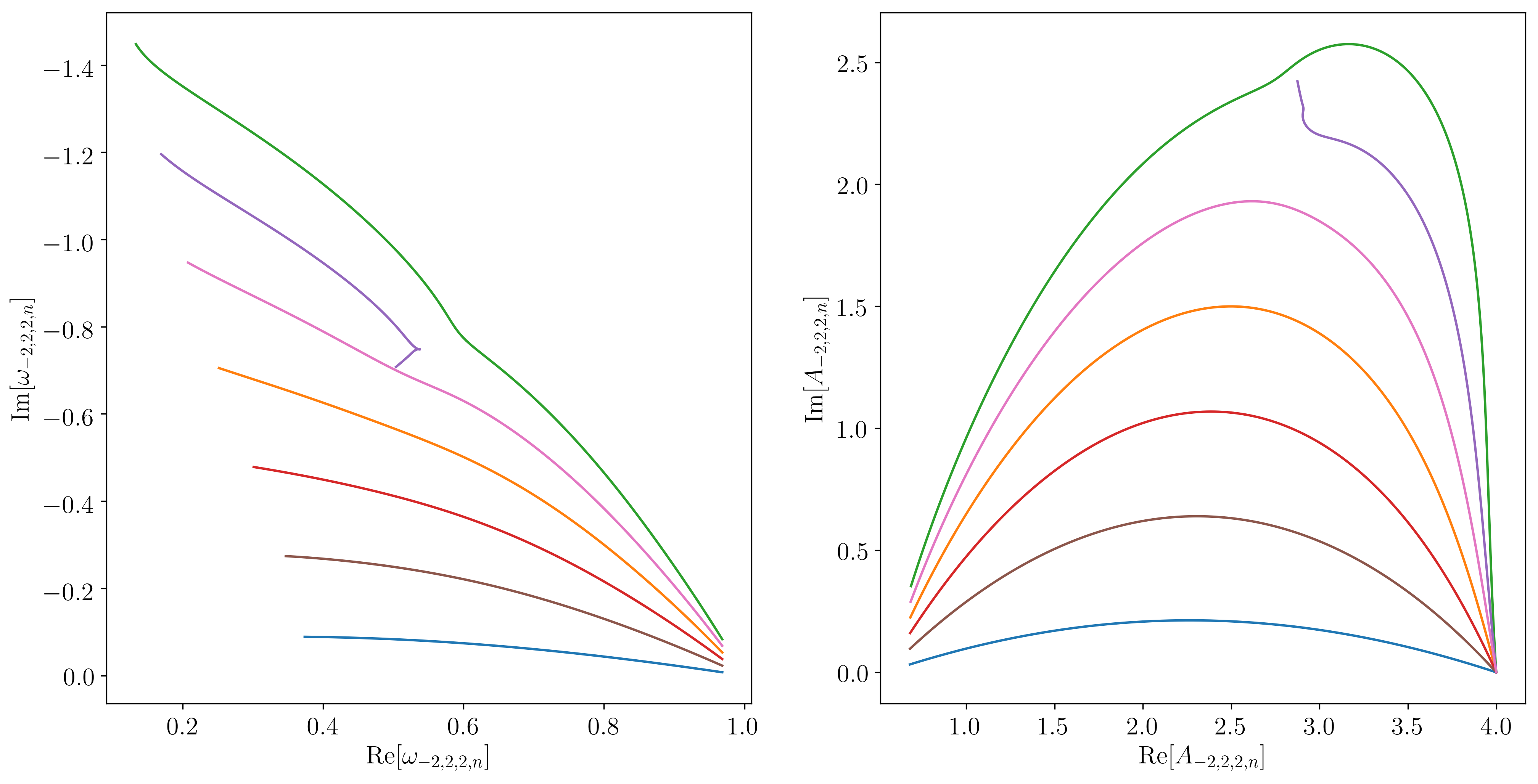_images/example_22n.png example_22n plot

s, l, n = (-2, 2, 0)
mode_list = [(s, l, m, n) for m in np.arange(-l,l+1)]
modes = {}
for ind in mode_list:
    modes[ind] = ksc(*ind)

plt.figure(figsize=(16,8))

plt.subplot(1, 2, 1)
for mode, seq in modes.items():
    plt.plot(np.real(seq.omega),np.imag(seq.omega))


modestr = "{},{},m,0".format(s,l)
plt.xlabel(r'$\textrm{Re}[\omega_{' + modestr + r'}]$', fontsize=16)
plt.ylabel(r'$\textrm{Im}[\omega_{' + modestr + r'}]$', fontsize=16)
plt.gca().tick_params(labelsize=16)
plt.gca().invert_yaxis()

plt.subplot(1, 2, 2)
for mode, seq in modes.items():
    plt.plot(np.real(seq.A),np.imag(seq.A))

plt.xlabel(r'$\textrm{Re}[A_{' + modestr + r'}]$', fontsize=16)
plt.ylabel(r'$\textrm{Im}[A_{' + modestr + r'}]$', fontsize=16)
plt.gca().tick_params(labelsize=16)

plt.show()

Which results in the following figure:

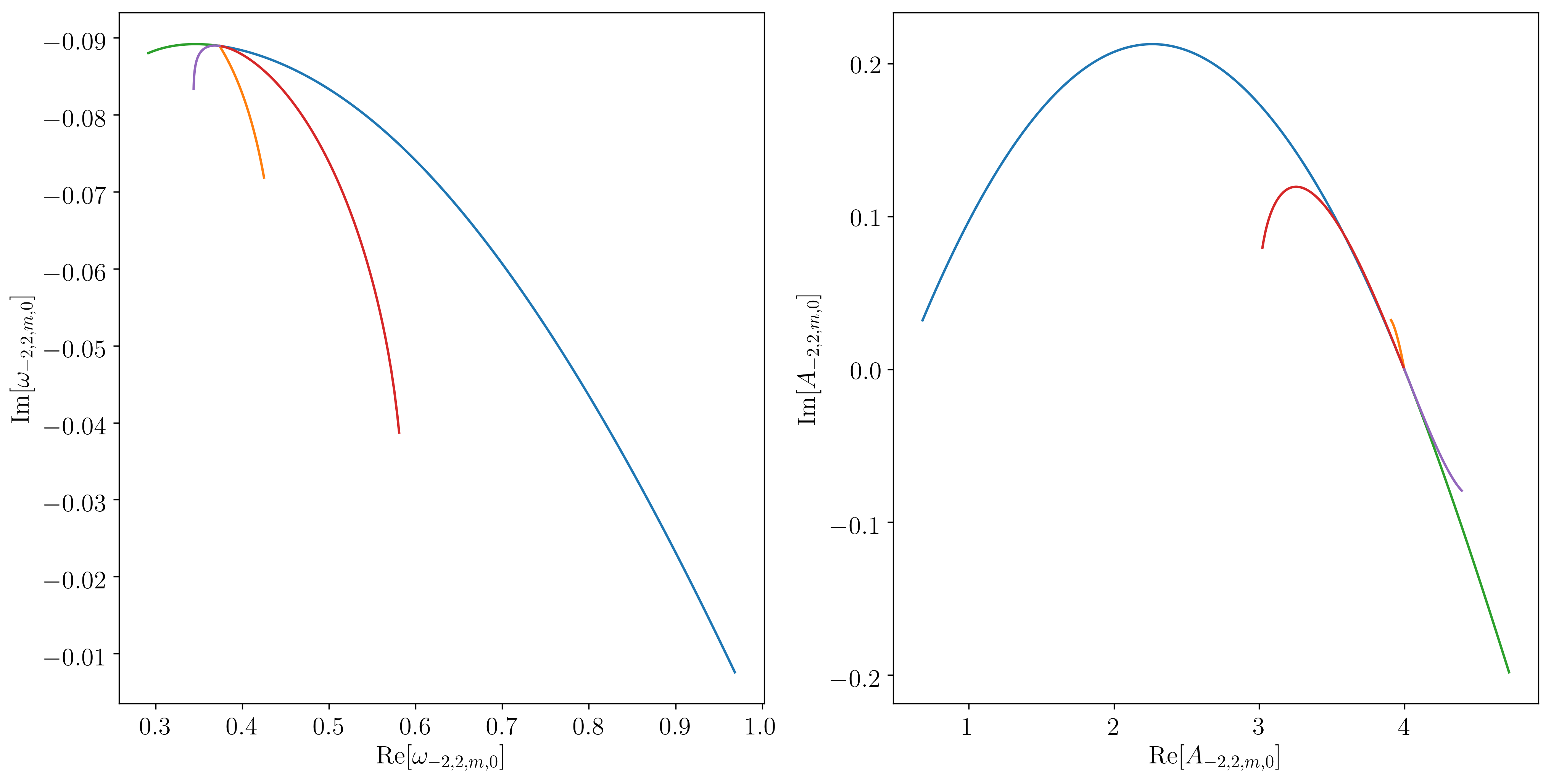_images/example_2m0.png example_2m0 plot

Credits¶

The code is developed and maintained by Leo C. Stein.